Computer Animation Week 4: Orientation

There are several ways to represent the orientation of an object in 3-dimensional space. Some important methods include Euler angles, coordinate frames, and quaternions.

Euler angles are values that represent the pitch, yaw, and roll of an object. These are angles that the object is rotated around on its local axes, as opposed to global axes. The yaw represents the angle than an object is rotated about its y-axis, the pitch is the angle it is rotated about its x-axis, and the roll is the angle it is rotated about its z-axis. This system has the advantage of being intuitive and easy to implement, but has the disadvantage of being susceptible to gimbal lock. Gimbal lock is the loss of one degree of freedom when two axes of rotation align in a parallel orientation, causing the object to only be able to rotate in two dimensions.

Coordinate frames are an important tool for defining the position and orientation of an object in 3-dimensional space. They work by defining an object’s direction vector (), up vector (), and right vector (). These vectors are all fairly self-explanatory; the direction vector points forward in the direction the object is facing, the up vector points up from the object, and the right vector points towards the right side of the object.  By combining these three vectors into a 3×3 matrix, [], we can fully define the orientation of the object. This can then combined with a vector that represents the object’s position in space (called ), creating a matrix which fully represents the object’s coordinate frame: []. We add an extra row ([0 0 0 1]) at the bottom to make it into a 4×4 matrix.

I will discuss quaternions in a later blog entry, but an extra topic I wanted to discuss this week is the Frenet frame. The Frenet frame, also known as TNB frame, is a method used in animation to determine the correct orientation of an object that is moving along a predetermined path, so that it will always be looking in the direction it is moving. This is done by looking ahead on the path by a small amount to find a point P2 that the object is moving towards, and subtracting the objects current position P1 from it. The result is then normalized, which produces a  vector for the object. The  vector is then created by calculating the cross product of  and the global up vector, . Finally, is calculated by taking the cross product of and . We then have all of the information needed to orientate the object correctly while it follows its path.

Object rotating according to the path it is following using a TNB frame. T stands for Tangent, and corresponds to the Direction vector (D). N stands for Normal, which corresponds to the Up vector (U). B stands for Bi-normal, which corresponds to the Right vector (R).

 

Computer Animation Week 3: Interpolation

Interpolation is the process of constructing new data points in the range of known data points. In computer animation, it allows us to create constant locomotion of objects between discrete waypoints. There are several different types of interpolation, but in class we discussed two main ones: linear interpolation (LERP), and splines.

Graph showing linear interpolation (LERP) between each red point.

Linear interpolation is the process of connecting waypoints by straight paths. As is seen in the image above, each waypoint, represented by red dots, is connected by blue lines that represent the interpolation between each way-point. This is the simplest form of interpolation, and the easiest to implement in code. However, as can be seen, it produces a curve that is not very smooth. While this is not so much of a problem for certain applications, for computer animation purposes it is generally not visibly appealing to see objects moving along paths that were generated via linear interpolation.

To calculate a linear interpolation, we use the term u to represent the current progress between the last waypoint and the next. For example, u would be 0.25 a quarter of the way to the second point, 0.5 exactly halfway between two points, and 0.75 three quarters of the way. The equation we can then use to calculate linear interpolation between point A and point B is:

p = (u – 1) * A + u * B

Where p is the point we are trying to calculate. This works in any number of dimensions, as each axis would be calculated independently.

As we discussed earlier, linear interpolation works well as a simple solution to find a straight path between waypoints, but is not great for generating a smooth path. This leads us to splines, the next form of interpolation that we discussed in class. Splines allow us to interpolate between waypoints in a way that produces a smooth curve across the entire path. There are several types of splines, but the two types we focused on in class were Bezier curves and Catmull-Rom splines.

A Bezier curve. P0 and P3 are the endpoints of the curve, while P1 and P2 are the control points.

A Bezier spline is specified by two endpoints and two control points. The location of the control points determines the curvature of the line that extends between the endpoints. The imaginary line that extends from an endpoint to its corresponding control point is the tangent at that very end of the curve, thus determining its slope at that endpoint.

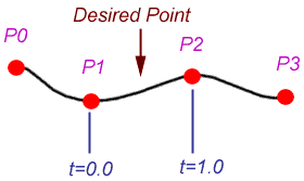
A Catmull-Rom spline.

A Catmull-Rom spline is similar to a Bezier spline, except that it does not have specific control points that are separate from the points on the curve. Rather, points act as control points for its neighbours, producing a smooth curve without needing to play around with control points.

Splines can be represented mathematically using the following formula:

Where u is the same as it was in linear interpolation, representing the progress from the current point to the next, p(u) is the value of position on the curve at u, and [pi-1 pi pi+1 pi+2] are the endpoints and control points on a Bezier spline, or the points surrounding the current point on a Catmull-Rom spline. M is a matrix of constants that is different for Bezier and Catmull-Rom splines. For Bezier splines, it is:

and for Catmull-Rom splines, it is: